ABC Analysis with Power Query

After an amazing first Power Query workshop in English, we are providing our attendees with even more CRAZY cool content that they’ll be able to put into practice (and understand) right away!

You might have already seen an ABC Classification Pattern with Power Pivot here, but this time you’re going to see this pattern being implemented with nothing but M code in Power Query.

Why? you might ask.

Is not only a simple and quick solution, in the case that you don’t want to use Power Pivot, but it also has some major feature advantages that can make truly unique solutions that could take you more time to implement in Power Pivot or they might end up adding unnecessary complexity to an already complex Data Model.

Let’s step into the solution and find out why this is a major step forward all Excel Users and even long-time Power Pivot users.

Concepts Covered

• Accessing data from a SQL Server Database
• Using custom Date Filters (show Last x days/months/years)
• Getting values and tables from related tables
• Grouping rows
• Using Lists
• Why you might consider using List.Buffer()
• Running Totals with Power Query
  • Using an Index Column or
  • The List.Select function
• Simple Conditional Logic with if

Our Data Source

First, we need to tell you that we’ll be using the Azure SQL Server that we provide to all of our attendees for this example. Within that server we have multiple databases, but the one that we’re going to use here is the AdventureWorks Database. If you are reading this and you went to one of our workshops then you already have the credentials to run this and if you have a version of the AdventureWorks database at hand then you can follow along as well.

Step 1: Get the Data

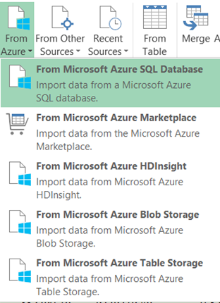
In the Power Query Ribbon, select From Azure and then select From Azure SQL Database. Enter the server and database info in order to connect to the data source.

You’ll then be prompted to enter your credentials with the correct authentication method. Once that happen, we’ll select the SalesOrderDetail Table from the list or simply use the search box to find it and once we click edit we’ll see that our table looks like this:

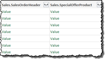
What we want to do first is a simply scroll all the way to the right and find the column with Values.

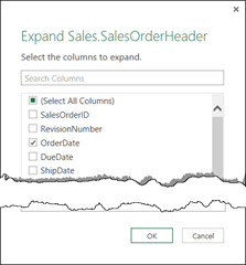
Once we find them, we’re going to expand them like this:

• On the Sales.SalesOrderHeader:
• On the Sales.SpecialOfferProduct:

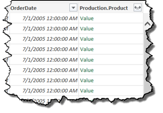
Once that happens, our result will give us 2 columns. One with the Date of the order and another one data related to the product sold:

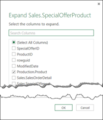
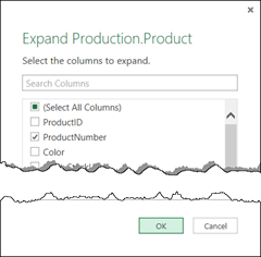
Let’s go ahead and expand that Product.Product column like this:

And once we’re done with the Table.ColumnExpand operations the result are 2 new columns: OrderDate and ProductNumber.

Step 2: Filter the Data using Date Filter

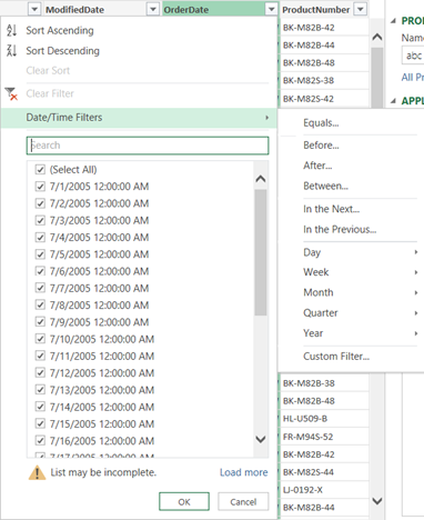
One of the relatively newer feature of Power Query are the Date/Time Filter:

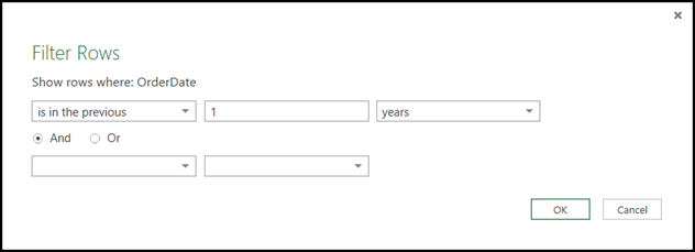
In our specific scenario, we want to add a  In the Previous.. filter, were we can always get an ABC Analysis based on the last month, year or perhaps on a specific amount of days. That dialogue windows is completely user friendly as well!

You could even have some even more complex calculations where you need to do Filtering at different levels like:

• Year-To-Date
• This Month
• This Week or more

By using this feature I’m making sure that I always get a more dynamic scenario where the ABC Analysis will be done against, let’s say, the last 52 weeks of sales data or perhaps just last year data and we could compare it again this year’s data (that could potentially take us a few simple clicks once we finish this solution if we wanted to!)

Step 3: Summarize the Data

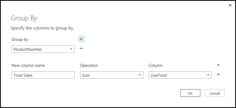
We’ve reached a point where we can simply group the data by the ProductNumber and simply have the total amount of sales for each product. We can do that by choosing the Group By feature from the Transform tab that will launch a new window with the following dialogue:

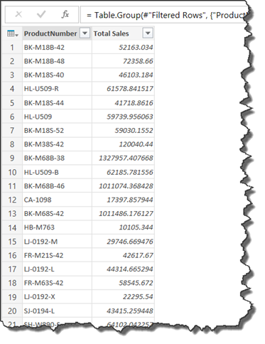
And the result of that Group By operation gives us the following table:

Step 4: Create a List of all the values to be considered

We simply add a Custom Step and add the following code to it (remember that you could right click the column and add a new step based on that column as a list):

• = List.Buffer(#”Grouped Rows”[Total Sales])

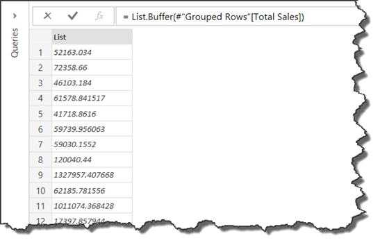
This creates a List with the values found in the Total Sales column of the previous step (Grouped Rows). We use List.Buffer for stability and to optimize performance as we’ll be using this later on. You might consider using List.Buffer in times like this where you might be using that list a few times and recalculating that List might hit you pretty bad in terms of performance. I also noticed that all the steps done prior to the Grouping By were not folded (as in not being used in the query folding), so everything from the Group By operation is now done locally at your computer.

The result of the previous operation gives us a List like the following:

Now that we’re done creating that list, we need to go back to where we were by adding another custom step. Click on the FX icon in the formula bar and add the name of your previous step as its shown in the image below:

Step 5: Add the Cumulative Column

There are many ways to create this cumulative column, but the 2 most efficient ones are:

• Using an Index column as a parameter combined with functions like List.Range, List.FirstN, List.Generate and then add the resultant list with functions like List.Sum or List Accumulate.
  • This often requires that you do a sorting prior to the previous step so you can get the data arranged in a descending or ascending way as required and it may often add some unnecessary steps or complexity.
• Using List.Select
  • The more straightforward way and it replicates what Marco and Alberto did with the EARLIER function in DAX

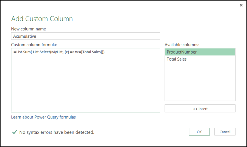
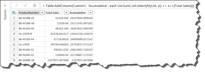
In our case, we’ll go with List.Select and add a new custom column like this:

Big thanks to Curt Hagenlocher from the MSFT Power Query team for helping me figure out the last few bits of this code. What it essentially does is basically take a List (in our case is the list we created before with the stepname MyList) and then only bring the rows that meet a certain criteria. That 2nd argument is actually a function where x is the value found at each row of the list and [Total Sales] is the value acting as the criteria.

So, in short, we’re basically calculating a new list on a row by row basis in our current table that is the result of filtering the MyList list where the value from the column [Total Sales] needs to be lower or equal to the values in the MyList. Once we have that output list, we simply use the List.Sum function to sum it and the result can be seen on the previous image. As you can see, we haven’t sorted that table and we already see some promising results.

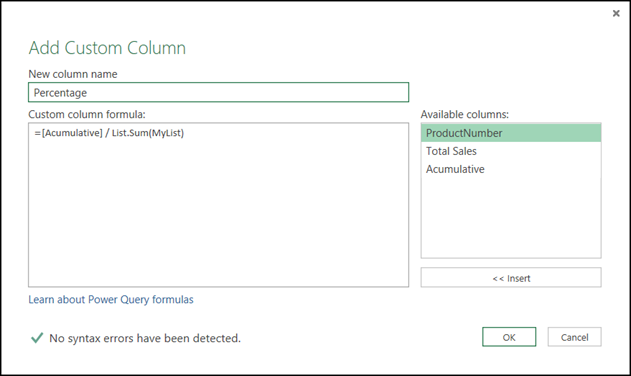
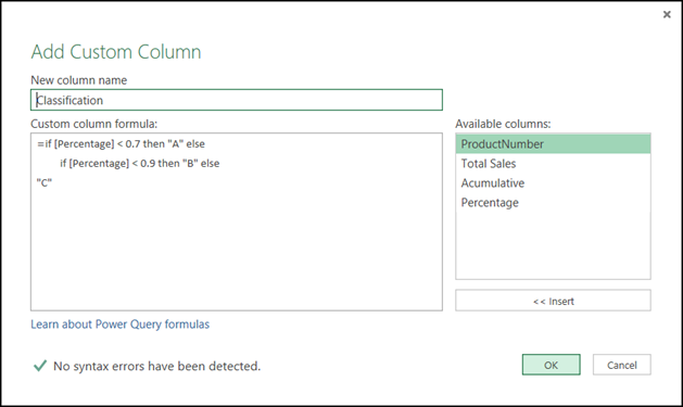
Step 6: Add the % and Classification column

We’re going to leave that sorting until the very end. For now, let’s focus on adding the needed columns using the following formulas:

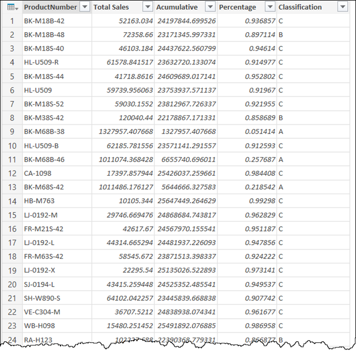
After adding those 2 custom columns, our Table should look like this:

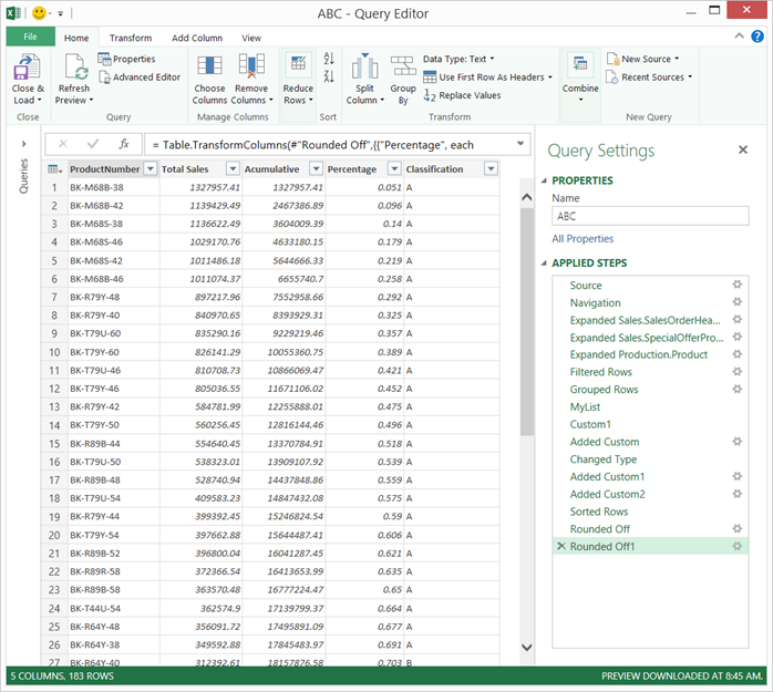
Step 7: Sorting & Rounding

We can now give in and sort the table as we want plus correct the decimals by rounding the numbers. The final result should look like this:

Other steps that we could do….

• We could potentially add more data related to the product by simply merging queries
• We could create multiple queries, 1 for each year or desired time-period,  and compare them all together
• We could load this Directly to our Data Model
• We could Group by Subcategory, Category or other attribute and do the ABC Analysis at that level

The Code

For the people that love looking at the code, I got you covered 🙂

let
    Source = Sql.Database(server, "AdventureWorks2012"),
    Sales_SalesOrderDetail = Source{[Schema="Sales",Item="SalesOrderDetail"]}[Data],
    #"Expanded Sales.SalesOrderHeader" = Table.ExpandRecordColumn(Sales_SalesOrderDetail, "Sales.SalesOrderHeader", {"OrderDate"}, {"OrderDate"}),
    #"Expanded Sales.SpecialOfferProduct" = Table.ExpandRecordColumn(#"Expanded Sales.SalesOrderHeader", "Sales.SpecialOfferProduct", {"Production.Product"}, {"Production.Product"}),
    #"Expanded Production.Product" = Table.ExpandRecordColumn(#"Expanded Sales.SpecialOfferProduct", "Production.Product", {"ProductNumber"}, {"ProductNumber"}),
    #"Filtered Rows" = Table.SelectRows(#"Expanded Production.Product", each Date.IsInPreviousNYears([OrderDate], 7)),
    #"Grouped Rows" = Table.Group(#"Filtered Rows", {"ProductNumber"}, {{"Total Sales", each List.Sum([LineTotal]), type number}}),
    MyList = List.Buffer(#"Grouped Rows"[Total Sales]),
    Custom1 = #"Grouped Rows",
    #"Added Custom" = Table.AddColumn(Custom1, "Acumulative", each List.Sum( List.Select(MyList, (x) => x>=[Total Sales]))),
    #"Changed Type" = Table.TransformColumnTypes(#"Added Custom",{{"Acumulative", type number}}),
    #"Added Custom1" = Table.AddColumn(#"Changed Type", "Percentage", each [Acumulative] / List.Sum(MyList)),
    #"Added Custom2" = Table.AddColumn(#"Added Custom1", "Classification", each if [Percentage] < 0.7 then "A" else
         if [Percentage] < 0.9 then "B" else
"C"),
    #"Sorted Rows" = Table.Sort(#"Added Custom2",{{"Total Sales", Order.Descending}}),
    #"Rounded Off" = Table.TransformColumns(#"Sorted Rows",{{"Total Sales", each Number.Round(_, 2)}, {"Acumulative", each Number.Round(_, 2)}}),
    #"Rounded Off1" = Table.TransformColumns(#"Rounded Off",{{"Percentage", each Number.Round(_, 3)}})
   in
    #"Rounded Off1"

Conclusion

Power Query is not just a tool for removing or renaming columns, unpivoting, grouping, appending or merging tables – it’s a full blown ETL tool that sits within the environment that you already know and love –Excel.

Mastering this tool is easier than mastering a language like VBA yet, you get more benefits from Power Query because it was designed from the ground-up to be a killer ETL tool.

The scenarios that you can solve with this tool are endless. During the upcoming weeks I’ll be posting more advanced scenarios with Power Query, so stay tuned and sign up for the newsletter on the right sidebar.

Don’t forget to visit the Power Query Training site for even more pattern, tricks and courses on Power Query.